Posterior inference in Bayesian Additive Regression Trees
Published:
In this post we will show how the posterior inference in BART is performed. To do this, we first introduce the specification of the likelihood for BART. Later, we show the algorithm Bayesian backfitting MCMC for posterior inference in BART used to sample from the posterior. Finally, we will briefly describe different approaches to sample the tree structure.
Likelihood specification for BART
As we commented in a previous post, BART is a sum-of-trees model specified by:
\[y=\sum_{j=1}^{m}g(x; T_j, M_j)+\epsilon\text{,}\qquad \epsilon \sim \mathcal{N}(0,\sigma^2)\text{.}\]To reduce clutter in the text, from now on, we will write $\{T_j, M_j\}_{j=1}^m$ to refer to $(T_1, M_1), \ldots,(T_m, M_m)$.
Hence, the likelihood for a training instance is
\[\ell\left ( y \mid \{T_j, M_j\}_{j=1}^m, \sigma, x \right ) = \mathcal{N} \left ( y \mid \sum_{j=1}^{m}g(x; T_j, M_j), \sigma \right )\]and the likelihood for the entire training dataset (note that $Y = (y_1, \ldots, y_n)$) is
\[\ell\left ( Y \mid \{T_j, M_j\}_{j=1}^m, \sigma, X \right ) = \prod_{i=1}^n \ell(y_i \mid \{T_j, M_j\}_{j=1}^m, \sigma, x_i)\text{.}\]Bayesian backfitting MCMC for posterior inference in BART
Given the likelihood and the prior, the posterior distribution is
\[p \left (\{T_j, M_j\}_{j=1}^m, \sigma \mid Y,X \right ) \propto \ell\left ( Y \mid \{T_j, M_j\}_{j=1}^m, \sigma, X \right ) p \left ( \{T_j, M_j\}_{j=1}^m , \sigma \mid X \right )\text{.}\]To sample from the BART posterior, Chipman et al. (2010) propposed a Bayesian backfitting MCMC algorithm. At a general level, this algorithm is a Gibbs sampler that loops through the trees, sampling:
- each tree $T_j$ and associated parameters $M_j$ conditioned on $\sigma$ and the remaining trees and their associated parameters, $\{ T_{j’}, M_{j’} \}_{j’\neq j}$; and
- $\sigma$ conditioned on all the trees and parameters $\{T_j, M_j\}_{j=1}^m$.
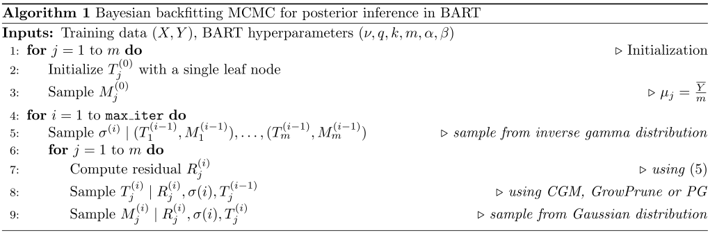
Let $T_j^{(i)}$, $M_j^{(i)}$, and $\sigma^{(i)}$ denote the values of $T_j$, $M_j$ and $\sigma$ at the $i^{th}$ MCMC iteration, respectively. Sampling $\sigma$ conditioned on $\{T_j, M_j\}_{j=1}^m$ is straightforward due to conjugacy, i.e., a draw from a inverse gamma distribution. To sample $T_j, M_j$ conditioned on the other trees $\{ T_{j’}, M_{j’} \}_{j’\neq j}$, we first sample $T_j \mid \{ T_{j’}, M_{j’} \}_{j’\neq j}, \sigma$ and then sample $M_j \mid T_j, \{ T_{j’}, M_{j’} \}_{j’\neq j}, \sigma$. More precisely, we compute the residual
\[R_j = Y - \sum_{j'=1, j'\ne j}^m g(X; T_{j'}, M_{j'})\text{.}\]Using the residual $R_j^{(i)}$ as the target, sample $T_j^{(i)}$ by proposing local changes to $T_j^{(i-1)}$. Finally, $M_j$ is sampled from a Gaussian distribution conditioned on $T_j, \{ T_{j’}, M_{j’} \}_{j’\neq j}, \sigma$. The algorithm is summarized in the following figure.
Sample of the tree structure, $T_j^{(i)} \mid R_j^{(i)}, \sigma^{(i)}, T_j^{(i-1)}$
To sample $T_j$, Chipman et al. (2010) use the MCMC algorithm proposed by Chipman et al. (1998). This algorithm, which we refer to as CGM, is a Metropolis-within-Gibbs sampler that randomly chooses one of the following four moves:
- grow: randomly chooses a leaf node and splits it further into left and right children,
- prune: randomly chooses an internal node where both the children are leaf nodes and prunes the two leaf nodes, thereby making the internal node a leaf node,
- change: changes the decision rule at a randomly chosen internal node,
- swap: swaps the decision rules at a parent-child pair where both the parent and child are internal nodes.
Another approach, introduced by Patrola et al. (2013) to reduce computational time, proposes using only the grow and prune moves; we will call this the GrowPrune sampler.
Finally, Lakshminarayanan et al. (2015) proposed a sampler based on the Particle Gibbs algorithm; we will call this PG. The PG sampler is implemented using the conditional SMC algorithm (instead of the Metropolis-Hastings sampler). Rather than making local changes to individual trees (as in Chipman et al. (2010)), the PG sampler proposes a complete tree to fit the residual.
References
- Chipman, H. A., George, E. I., & McCulloch, R. E. (2010). BART: Bayesian additive regression trees. The Annals of Applied Statistics, 4(1), 266-298.
- Lakshminarayanan, B., Roy, D., & Teh, Y. W. (2015, February). Particle Gibbs for Bayesian additive regression trees. In Artificial Intelligence and Statistics (pp. 553-561).
- Kapelner, A., & Bleich, J. (2013). bartMachine: Machine learning with Bayesian additive regression trees. arXiv preprint arXiv:1312.2171.
- Tan, Y. V., & Roy, J. (2019). Bayesian additive regression trees and the General BART model. arXiv preprint arXiv:1901.07504.
- Chipman, H. A., George, E. I., & McCulloch, R. E. (1998). Bayesian CART model search. Journal of the American Statistical Association, 93(443), 935-948.
- Pratola, M. T., Chipman, H. A., Gattiker, J. R., Higdon, D. M., McCulloch, R., & Rust, W. N. (2014). Parallel Bayesian additive regression trees. Journal of Computational and Graphical Statistics, 23(3), 830-852.