Introduction

Bayesian Additive Regression Trees (BART) is a sum-of-trees model for approximating an unknown function $f$. Like other ensemble methods, every tree act as a weak learner, explaining only part of the result. All these trees are of a particular kind called decision trees. The decision tree is a very interpretable and flexible model but it is also prone to overfitting. To avoid overfitting, BART uses a regularization prior that forces each tree to be able to explain only a limited subset of the relationships between the covariates and the predictor variable.

The problem BART tackles is making inference about an unknown function $f$ that predicts an output $y$ using a $p$ dimensional vector of inputs $x=(x_1,\ldots,x_p)$ when

To solve this regression problem, BART approximates $f(x)=E(y \mid x)$ using $f(x)\approx h(x)\equiv \sum_{j=1}^{m}g_j(x)$, where each $g_j$ denotes a regression tree:

The BART model

The BART model consists of two parts: a sum-of-trees model and a regularization prior on the parameters of that model.

A sum-of-trees model

To elaborate the form of the sum-of-trees model (\ref{general-sum-of-tree-model}), we begin by establishing notation for a single tree model. Let $T$ denote a binary tree consisting of a set of interior node decision rules and a set of terminal nodes, and let $M=\{\mu_1, \mu_2, \ldots, \mu_b\}$ denote a set of parameter values associated with each of the $b$ terminal nodes of $T$. The decision rules are binary splits of the predictor space of the form $\{x \in A\}$ vs $\{x \notin A\}$ where $A$ is a subset of the range of $x$. These are typically based on the single components of $x = (x_1, \dots , x_p)$ and are of the form $\{x_i \leq c\}$ vs $\{x_i > c\} $ for continuous $x_i$. Given the way it is constructed, the tree is a full binary tree, that is, each node has exactly zero or two children. Each $x$ value is associated with a single terminal node of $T$ by the sequence of decision rules from top to bottom, and is then assigned the $\mu_i$ value associated with this terminal node. For a given $T$ and $M$, we use $g(x; T, M)$ to denote the function which assigns a $\mu_i \in M$ to $x$.

With this notation, the sum-of-trees model (\ref{general-sum-of-tree-model}) can be more explicitly expressed as:

where for each binary regression tree $T_j$ and its associated terminal node parameters $M_j$, $g(x; T_j, M_j)$ is the function which assigns $\mu_{ij} \in M_j$ to $x$. Under (\ref{well-specified-sum-of-tree-model}), $E(y \mid x)$ equals the sum of all the terminal node $\mu_{ij}$’s assigned to $x$ by the $g(x; T_j, M_j)$’s.

The following image is an example of $g(x; T_j, M_j)$,

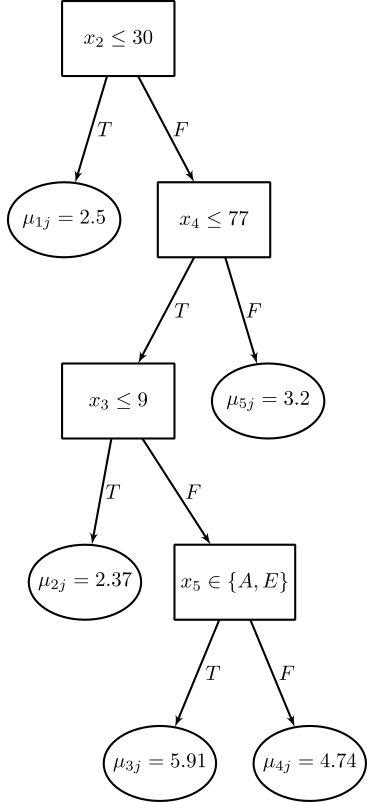
Each such $\mu_{ij}$ will represent a main effect when $g(x; T_j, M_j)$ depends on only one component of $x$ (i.e., single variable), and will represent an interaction effect when $g(x; T_j, M_j)$ depends on more than one component of $x$ (i.e., more than one variable). Thus, the sum-of-trees model can incorporate both main effects and interaction effects. And because (\ref{well-specified-sum-of-tree-model}) may be based on trees of varying sizes, the interaction effects may be of varying orders. In the special case where every terminal node assignment depends on just a single component of $x$, the sum-of-trees model reduces to a simple additive function, a sum of step functions of the individual components of $x$.

With a large number of trees, a sum-of-trees model gains increased representation flexibility which endows BART with excellent predictive capabilities. This representational flexibility is obtained by rapidly increasing the number of parameters. Indeed, for fixed $m$, each sum-of-trees model (\ref{well-specified-sum-of-tree-model}) is determined by $(T_1, M_1), \ldots,(T_m, M_m)$ and $\sigma$, which includes all the bottom node parameters as well as the tree structures and decision rules.

A regularization prior

The BART model specification is completed by imposing a prior over all the parameters of the sum-of-trees model, namely, $(T_1, M_1), \ldots,(T_m, M_m)$ and $\sigma$. There exists specifications of this prior that effectively regularize the fit by keeping the individual tree effects from being unduly influential. Without such a regularizing influence, large tree components would overwhelm the rich structure of (\ref{well-specified-sum-of-tree-model}), thereby limiting the advantages of the additive representation both in terms of function approximation and computation.

Chipman et al. proposed a prior formulation in term of just a few interpretable hyperparameters which govern priors on $T_j$, $M_j$ and $\sigma$. When domain information is not available the authors recomend using an empirical Bayes approach and calibrate the prior using the observed variation in $y$. Or at least to obtaing a range of plausible values and the perform cross-validation to select from these values.

Prior independence and symmetry

In order to simplify the specification of the regularization prior we restrict our attention to priors for which the tree components ($T_j$, $M_j$) are independent of each other and also independent of $\sigma$, and the terminal node parameters of every tree are independent.

\begin{equation} \begin{split} p((T_1 , M_1), \ldots , (T_m , M_m ), \sigma ) &= \left [ \prod_j p(T_j , M_j) \right ] p(\sigma)\\ &= \left [ \prod_j p(M_j \mid T_j) p(T_j) \right ] p(\sigma) \end{split} \end{equation}

and

where $\mu_{ij} \in M_j$.

Under the independence assumption we only need to specify $p(T_j)$, $p(\mu_{ij} \mid T_j)$ and $p(\sigma)$.

The $T_j$ prior

The $T_j$ prior, $p(T_j)$, is specified by three aspects:

• the probability that a node at depth $d=(0, 1, 2, \ldots)$ is nonterminal, given by: $ \frac{\alpha}{(1 + d)^{\beta}}$ with $\alpha \in (0, 1)$ and $\beta \in \lbrack 0, \infty)$. Node depth is defined as distance from the root. Thus, the root itself has depth $0$, its first child node has depth $1$, etc. This prior controls the tree depth. For a sum-of-trees model with $m$ large, we want the regularization prior to keep the individual tree components small. To do that, we usually use $\alpha=0.95$ and $\beta=2$. Even though this prior puts most probability on tree sizes of $2$ or $3$, trees with many terminal nodes can be grown if the data demands it.
• the distribution on the splitting variable assignments at each interior node. Usually, this is the uniform prior on available variables
• the distribution on the splitting rule assignment in each interior node, conditional on the splitting variable. Usually, this is the uniform prior on the discrete set of available splitting values.

The $\mu_{ij} \mid T_j$ prior

For convenience, we first shift and rescale $y$ so that the observed transformed values range from $y_{min} = -0.5$ to $y_{max} = 0.5$, then the prior is

where $\sigma_{\mu} = \frac{0.5}{k\sqrt{m}}$.

This prior has the effect of shrinking the tree parameters $\mu_{ij}$ toward zero, limiting the effect of the individual tree components by keeping them small. Note that as $k$ and/or $m$ is increased, this prior will become tighter and apply greater shrinkage to the $\mu_{ij}$. Chipman et al. (2010) found that a value of $k$ between $1$ and $3$ yield good results.

The $\sigma$ prior

We used the inverse chi-square distribution

Essentially, we calibrate the prior for the degree of freedom $\nu$ and scale $\lambda$ for this purpose using a rough data-based overestimate $\hat \sigma$ of $\sigma$. Two natural choices for $\hat \sigma$ are:

• the naive specification, in which we take $\hat \sigma$ to be the sample standard deviation of $y$
• the linear model specification, in which we take $\hat \sigma$ as the residual standard deviation from a least squares linear regression of $y$ on the original $X$.

We then pick a value of $\nu$ between $3$ and $10$ to get an appropriate shape, and a value of $\lambda$ so that the $q$th quantile of the prior on $\sigma$ is located at $\hat \sigma$, that is, $P(\sigma < \hat \sigma) = q$. We consider values of $q$ such as $0.75$, $0.90$ or $0.99$ to center the distribution below $\hat \sigma$.

For automatic use, Chipman et al. (2010) recommend the default setting $(\nu, q) = (3, 0.90)$. It is not recommended to choose $\nu < 3$ because it seems to concentrate too much mass on very small $\sigma$ values, which leads to overfitting.

The choice of $m$

Instead of being fully Bayesian and estimate the value of $m$, a fast and robust option is to choose $m=200$ and then maybe check if a couple of other values makes any difference. As $m$ is increased, starting with $m = 1$, the predictive performance of BART improves dramatically until at some point it levels off and then begins to very slowly degrade for large values of $m$. Thus, for prediction, it seems only important to avoid choosing $m$ too small.

Inference

Given the observed data $y$, the Bayesian setup induces a posterior distribution

on all the unknowns that determine a sum-of-trees model (\ref{well-specified-sum-of-tree-model}). Although the sheer size of the parameter space precludes exhaustive calculation, Chipman et al. (2010) propose a backfitting MCMC algorithm that can be used to sample from this posterior. On the other hand, Lakshminarayanan et al. (2015) show that Particle Gibbs is a better approach for Bayesian Additive Regression Trees. In a future post, we’ll talk more about this.

Results

The ouput of a BART model is:

• a posterior mean estimate of $f(x) = E(y \mid x)$ at any input value $x$
• pointwise uncertainty intervals for $f(x)$
• variable importance meassures. This is done by keeping track of the relative frequency with which $x$ components appear in the sum-of-trees model iterations.

References

1. Chipman, H. A., George, E. I., & McCulloch, R. E. (2010). BART: Bayesian additive regression trees. The Annals of Applied Statistics, 4(1), 266-298.
2. Lakshminarayanan, B., Roy, D., & Teh, Y. W. (2015). Particle Gibbs for Bayesian additive regression trees. In Artificial Intelligence and Statistics (pp. 553-561).
3. Kapelner, A., & Bleich, J. (2013). bartMachine: Machine learning with Bayesian additive regression trees. arXiv preprint arXiv:1312.2171.
4. Chipman, H. A., George, E. I., & McCulloch, R. E. (1998). Bayesian CART model search. Journal of the American Statistical Association, 93(443), 935-948.
5. Tan, Y. V., & Roy, J. (2019). Bayesian additive regression trees and the General BART model. arXiv preprint arXiv:1901.07504.